PolarQuant + QJL: The Two-Stage Secret Behind TurboQuant's Zero Loss
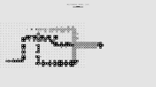
PolarQuant and QJL are the two algorithmic ideas behind the TurboQuant approach described by Google Research. PolarQuant prepares high-dimensional vectors for low-bit representation. QJL, short for Quantized Johnson-Lindenstrauss, handles a small residual signal with a one-bit sign representation and an estimator for downstream score calculations.
That division of work matters because quantization is not only a matter of choosing a smaller number of bits. A system must also manage vector geometry, scale information, estimation error, kernel support, and the quality metric that the application actually cares about. TurboQuant is presented as a method for key-value cache compression and vector search, not as a universal replacement for every quantization workflow. See our earlier TurboQuant analysis.
Google Research published its TurboQuant announcement on March 24, 2026. The announcement reports experiments on long-context benchmarks and describes a 3-bit configuration for KV cache work, plus an operation-level result in which 4-bit TurboQuant reached up to 8x performance for attention-logit computation over 32-bit unquantized keys on H100 accelerators. The results are tied to the reported configurations.
What You'll Learn
- Why TurboQuant uses a preparation stage and a residual stage.
- How random rotation and polar coordinates help PolarQuant.
- What QJL contributes to one-bit residual estimation.
- How to read the reported memory, benchmark, and speed results.
Why TurboQuant Uses Two Stages
A vector contains many numerical coordinates. Some coordinates may carry most of the magnitude while others carry directional detail. If a quantizer treats every coordinate in the same way, it can spend bits inefficiently or introduce an error that matters to the final dot product.
A two-stage design separates the main signal from the remaining error. The first stage aims to encode the dominant structure with a useful low-bit representation. The second stage handles a smaller residual. This does not mean the original floating-point vector is reconstructed exactly in every setting. It means the compressed representation is evaluated by the task that uses it.
For KV cache compression, the task is attention. The system needs the compressed keys and values to preserve the information used when a query selects relevant earlier tokens. For vector search, the task is similarity ranking. The system needs nearby candidates to remain near enough to appear in the retrieved set.
| Stage | Input or role | Evaluation question |
|---|---|---|
| Vector preparation | High-dimensional source vector | Can the geometry be made easier to represent? |
| Low-bit quantization | Main signal after transformation | How much memory is saved for the useful information? |
| Residual estimation | Small error left by the first stage | Does the score calculation retain task quality? |
| Serving kernel | Compressed data during inference or search | Does the implementation improve actual latency? |
Stage One: What PolarQuant Does
PolarQuant is the component Google describes as the high-quality compression stage. It uses a random rotation before quantization. The rotation changes the coordinate system without changing the underlying vector relationships. Its purpose is to spread the vector's energy so that one coordinate does not dominate the representation.
After rotation, PolarQuant uses a polar transformation. In a simple two-dimensional analogy, a point can be expressed by a radius and an angle instead of separate horizontal and vertical coordinates. In a high-dimensional method, the transformation is more involved. The practical idea is that magnitude and direction may follow patterns that are easier to quantize than raw coordinates.
Google's explanation says PolarQuant uses recursive polar transformations. The radius captures the strength of the vector and the angles capture directional information. A fixed angular structure can reduce the need to store a separate normalization value for every small block. That can leave more of the bit budget available for the data itself.
Random Rotation Before Quantization
Random rotation is a linear change of basis. It does not add information and it does not remove information from the source vector by itself. It presents the same vector in a different coordinate system before the quantizer sees it.
The reason to rotate is distribution. High-dimensional data can have uneven coordinate ranges. One dimension may have a large spread while another stays close to zero. A simple scalar quantizer then faces different scale requirements across coordinates. A random rotation can spread energy across dimensions and make the distribution more suitable for a shared representation.
This step should not be confused with random noise. The rotation is part of the mathematical transform. Its value is useful only if the decoder or score calculation uses the corresponding transform correctly. An implementation must keep the transform convention consistent across storage, retrieval, and computation.
Polar Coordinates and Quantization Overhead
Traditional vector quantization often stores values in blocks. Each block may need a scale or another constant that tells the decoder how to map a compact code back into a numerical range. These constants use memory. If a block is small, the metadata can take a meaningful share of the total representation.
PolarQuant addresses this issue through the geometry of the transformed vector. Google describes the angular pattern as concentrated and predictable. A fixed circular structure can reduce the need for repeated normalization information. The result is not a claim that metadata disappears from every implementation. It is a design intended to reduce hidden overhead.
The practical comparison is therefore not only 3 bits against 4 bits or 8 bits. Engineers should compare total bytes, including scales, codebooks, alignment, padding, and temporary buffers. They should also measure the time needed to apply the transform and the time needed to read the compact representation.
| Representation detail | Why it exists | What to measure |
|---|---|---|
| Magnitude or radius | Captures vector strength | Distribution and quantization error |
| Angular coordinates | Captures direction or orientation | Similarity and attention-score stability |
| Scale information | Maps compact codes to numerical ranges | Bytes per block and decode cost |
| Transform metadata | Keeps encoding and score calculation aligned | Storage, bandwidth, and kernel overhead |
Stage Two: What QJL Contributes
QJL is the residual stage in Google's description of TurboQuant. The method is related to the Johnson-Lindenstrauss idea of preserving useful relationships while mapping high-dimensional data into a smaller representation. Google describes QJL as reducing each resulting value to a sign bit, conceptually represented as plus one or minus one.
A one-bit signal is compact, but it can introduce bias. QJL uses an estimator that balances a higher-precision query with low-precision stored data. The goal is to estimate the attention score accurately enough for the application even though the cached representation uses far fewer bits.
QJL is therefore not simply a second copy of the first quantizer. It changes how the remaining error is represented and how the downstream score is calculated. A serving implementation must support that estimator. Storing sign bits without the matching score computation would not reproduce the method described by Google Research.
How the Residual Stage Affects Attention
During language-model generation, a query is compared with stored keys to determine which earlier information matters. The attention score depends on the relationship between the query and each key. Small numerical errors can be harmless in one context and important in another if they change the ranking of candidates.
The residual stage aims to protect the part of the relationship that the first stage did not capture. The estimator can use a more precise query and compact stored information. This is a different trade-off from reconstructing every cached value in full precision.
Quality testing should examine the final task. Perplexity can reveal a broad distribution change, while retrieval tasks can show whether a specific item remains accessible in a long context. A system that passes one test may still need a fallback for another task.
Bit Width Is Not the Whole Memory Calculation
Bit width describes how many bits represent a value or code under a defined convention. It does not by itself determine total memory. A real cache also contains dimensions, sequence positions, batch entries, alignment, metadata, and runtime buffers.
The same caution applies when comparing a 3-bit configuration with a 4-bit configuration. The 4-bit result in Google's announcement concerns attention-logit performance on H100 hardware. The 3-bit result concerns compact representation and benchmark outcomes in the reported KV cache experiments. They should not be merged into one claim that every configuration has the same speed and memory behavior.
| Claim type | Reported context | Safe reading |
|---|---|---|
| 3-bit cache representation | TurboQuant KV cache experiments | A low-bit configuration tested by Google Research |
| At least 6x memory reduction | Discussed needle-in-a-haystack results | A reported result for the tested comparison |
| Up to 8x performance | 4-bit attention logits over 32-bit keys on H100 | An operation-level hardware-specific result |
| No training or fine-tuning | Google's description of the method | Lower model-preparation burden, not zero integration work |
What Google Research Tested
Google reports experiments across LongBench, Needle In A Haystack, ZeroSCROLLS, RULER, and L-Eval. The announcement says the tests used open-source Gemma and Mistral models. These benchmarks cover long-context retrieval, question answering, code generation, summarization, and related tasks.
In its discussion of needle-in-a-haystack results, Google says TurboQuant reached perfect downstream results across the reported benchmarks while reducing KV memory by at least 6x. This is an experimental statement from the cited source. It does not establish that every model, language, prompt style, or context length will behave the same way.
Google also reports vector-search experiments using the 1@k recall ratio on the GloVe dataset with vector dimension 200. That result is relevant to search ranking, while an LLM cache test is relevant to attention and generation. The metrics should remain separate when the findings are summarized.
KV Cache and Vector Search Are Different Workloads
KV cache compression runs inside a generation loop. The cache is updated as tokens arrive and read as the model calculates attention. The serving path is sensitive to memory bandwidth, kernel launch cost, sequence length, and the number of concurrent requests.
Vector search stores embeddings in an index and compares a query with candidates. The main quality question is whether the correct nearest results remain in the returned set. The index-building path and the query path may have different limits.
A shared quantization method can serve both workloads, but the acceptance test must be different. An LLM team may focus on long-context retrieval and output quality. A search team may focus on recall, index size, query latency, and update cost.
For broader infrastructure context, read our AI agent ROI guide. Our AI builder guide covers application choices, while the model comparison guide covers model-level tradeoffs.
Why No Retraining Is Useful
Google says TurboQuant can quantize the KV cache without training or fine-tuning. That makes the method easier to test with an existing model because a team does not need to create a new weight checkpoint for the first experiment.
No retraining does not mean no software work. The runtime needs a compatible cache layout, a quantization path, an attention or similarity kernel, memory management, and a fallback. The team also needs tests that compare the compressed path with the existing precision format. Our TurboQuant implementation guide covers these testing limits in more detail.
A no-training method can shorten the experiment cycle. It does not remove the need to decide which requests use low-bit cache, which requests use a higher-precision fallback, and how the service reports a failure or quality threshold breach.
How to Validate PolarQuant and QJL in Production
Start with a fixed baseline. Record the model, weight format, cache format, context length, batch size, accelerator, kernel version, and task metrics. Then run the same request set against the compressed and baseline paths.
Measure memory and quality first. Capture peak allocation, active sequence count, long-context retrieval, perplexity where useful, and task-specific output checks. After that, measure prompt processing, token generation, attention time, and total request latency separately.
Include short prompts and long prompts. Include one request and a mixed batch. Include traffic that contains the languages, code, retrieval patterns, and safety controls used by the service. A method that helps one workload may need a different bit width or fallback for another.
| Validation area | Baseline comparison | Pass condition |
|---|---|---|
| Quality | Task scores, retrieval, perplexity | Within the service's accepted change range |
| Memory | Peak cache bytes and active requests | Capacity improves under real traffic shapes |
| Latency | Prefill, decode, and end-to-end time | Low-bit work helps the actual service path |
| Fallback | Unsupported shapes and quality failures | Requests remain available and diagnosable |
Conclusion: Read the Two Stages as a System
PolarQuant and QJL solve different parts of the low-bit representation problem. PolarQuant changes the geometry of a vector and prepares its main signal for compact storage. QJL uses a one-bit residual idea and an estimator to reduce bias in the downstream score. The two stages are connected by the workload that consumes the result.
Google Research reports strong findings for TurboQuant, including at least 6x KV memory reduction in the discussed retrieval results and up to 8x performance for a specific attention-logit configuration on H100 hardware. Those results justify controlled testing. They do not justify treating perfect reconstruction or universal zero loss as a guarantee for every deployment.
Engineers should compare total memory, quality, latency, and fallback behavior. The useful question is whether the two-stage design improves the target service while staying inside its quality and reliability limits.
Frequently Asked Questions

SK Jabedul Haque
Building India's most trusted finance education platform — simplifying news, schemes and market trends so anyone can understand and invest confidently.
Read full bio

Never miss an update
Get our clearest explainers on schemes, markets and money — read what matters, without the noise.
Explore more articles